2.3 An Example

We now consider the small example problem,

$${\rm minimize} \;\;\; F(x_1, x_2,x_3) \equiv x_1^2 + x_2^4 x_3^4 + x_2 \sin(x_1 + x_3) + x_1 x_3 + x_2$$

subject to the bounds $- 1 \leq x_2 \leq 1$ and $1 \leq x_3 \leq 2$. There are a number of ways of casting this problem in the form (2.1). Here, we consider partitioning $F$ into groups as

$$\begin{array}{ccccc} (x_1)^2 & + & (x_2 x_3)^4 & + & (x_2 \si... ...box{group 1} & & \mbox{group 2} & & \mbox{group 3} \end{array}$$

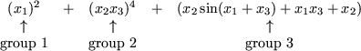
Notice the following:

1. group 1 uses the non-trivial group function $g_1 (\alpha) = \alpha^ 2$. The group contains a single linear element; the element function is $x_1$.

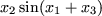
2. group 2 uses the non-trivial group function $g_2(\alpha) = \alpha^4$. The group contains a single nonlinear element; this element function is $x_2 x_3$. The element function has two elemental variables, $v_1$ and $v_2$, say, (with $v_1 = x_2$ and $v_2 = x_3$) but there is no useful transformation to internal variables.

3. group 3 uses the trivial group function $g_3 (\alpha) = \alpha$. The group contains two nonlinear elements and a single linear element $x_2$. The first nonlinear element function is $x_2 \sin ( x_1 + x_3 )$. This function has three elemental variables, $v_1$, $v_2$ and $v_3$, say, (with $v_1 = x_2$, $v_2 = x_1$ and $v_3 = x_3)$, but may be expressed in terms of two internal variables $u_1$ and $u_2$, say, where $u_1 = v_1$ and $u_2= v_2 + v_3$. The second nonlinear element function is $x_1 x_3$, which has two elemental variables $v_1$ and $v_2$ (with $v_1 = x_1$ and $v_2 = x_3$) and is of the same type as the nonlinear element in group 2.

Thus we see that we can consider our objective function to be made up of three groups; the first and second are non-trivial (and of different types) so we will have to provide our optimization procedure with function and derivative values for these at some stage. There are three nonlinear elements, one from group two and two more from group three. Again this means that we shall have to provide function and derivative values for these. The first and third nonlinear element are of the same type, while the second element is a different type. Finally one of these element types, the second, has a useful transformation from elemental to internal variables so this transformation will need to be set up.